
极简`Transformer`实现(基于`llama2.c`commit-4e23ad 23'7/27)
基于源码调试过程,以及如下两篇文章整理。
This repo is line by line walk through of the inference file in llama2.c. Its very verbose & intended for beginners.
You will need some familiarity with transformers architecture. If you are a complete novice refer to this excellent blog first.
The Illustrated Transformer。
llama2.c 包含了训练代码和推理实现,作者提供了如下几个预训练模型,可以直接运行 run 这个demo程序生成一个简短的小故事。
| model | dim | n_layers | n_heads | n_kv_heads | max context length | parameters | val loss | download |
|---|---|---|---|---|---|---|---|---|
| 260K | 64 | 5 | 8 | 4 | 512 | 260K | 1.297 | https://huggingface.co/karpathy/tinyllamas/tree/main/stories260K |
| OG | 288 | 6 | 6 | 6 | 256 | 15M | 1.072 | https://huggingface.co/karpathy/tinyllamas/resolve/main/stories15M.bin |
| 42M | 512 | 8 | 8 | 8 | 1024 | 42M | 0.847 | https://huggingface.co/karpathy/tinyllamas/resolve/main/stories42M.bin |
| 110M | 768 | 12 | 12 | 12 | 1024 | 110M | 0.760 | https://huggingface.co/karpathy/tinyllamas/resolve/main/stories110M.bin |
与一般的问答式文本生成不一样, run 的实现做了简化,首先是没有prompt 输入而是每次运行直接生成一个tiny story,所以也就没有针对prompt 做embedding 的 init_prefill 计算阶段,而只有 generate;其次是在生成的迭代过程中,主要的transformer计算输入输出只需要词元的 token 因此预先把所有词元的embedding存储在token_embedding_table 中,迭代过程中直接从里面读取当前位置的 embedding 参与计算,推理过程中可以省掉输入词元的embedding计算过程。
涉及到的输入文件有模型checkpoint如 stories15M.bin ,以及tokenizer 文件 tokenizer.bin ,具体的文件结构可以参考文末的分析。
执行流程
main处理命令行参数,模型推理主要在transformer函数里面。
main 执行流程
- 解析命令行参数,包括 checkpoint 文件路径, temperature, steps
- 加载checkpoint 文件内容,包括模型配置和权重
- 加载
tokenizer.bin - 初始化运行时变量,包括kv cache等
- 根据给定的 seq_len (steps) 执行循环,以 BOS 作为第一个token开始:
transformer 输出下一个token的logits
参考temperature的值,由logits得到token值
- 如果temperature==0,采用贪心搜索直接取最大值,$next=argmax(logits)$
- 否则,随机采样得到token,$next=sample(softmax(logits/temperature))$
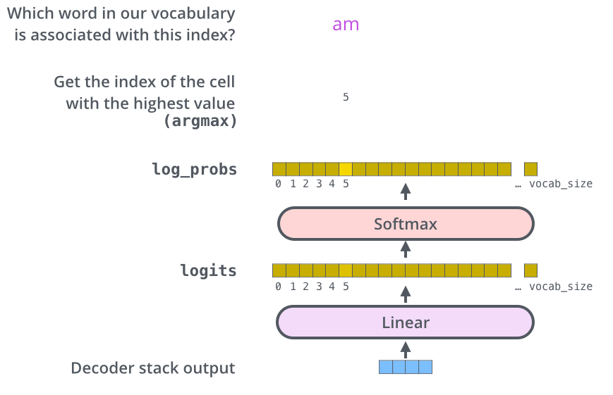
token即为vocab的index,从tokenizer中得到对应的单词并打印
- 内存清理并退出
transformer执行流程
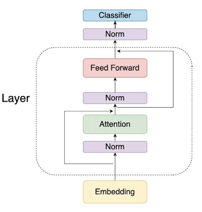
注意:因为是纯推理,所以实现的是decoder部分,att计算的是
Masked Multi-Head Attention,也就是代码中的[0, pos]相当于是mask之后的。
计算过程:
- 从
token_embedding_table中取出当前token的embedding (dim, ) 放入s->x中 - 循环遍历每一层:
对
s->x计算rmsnorm并存入s->xb对
s->xb计算 Q、K、V,结果存入s->q,s->k,s->v对每个多头,计算RoPE编码的Q、K,结果存入
s->q,s->k保存当前位置的KV到缓存
s->key_cache,s->value_cache注意K是带位置编码信息的,而V不带kv cache (layer, seq_len, dim),则
int loff = l * p->seq_len * dim是第l层的kv cache起始位置计算多头注意力,循环遍历每个头
- Q起始位置,Q(dim, 1)拆分多头后维度为(n_heads, head_dim),所以第
h头的起始位置为**float* q = s->q + h * head_size - atten score (n_heads, seq_len),因为是按头维度存放的,所以在第
h头的起始位置就是s->att + h * p->seq_len - kv cache在
dim维度拆分多头后为(layer, seq_len, n_heads, head_dim),则第h头的偏移为h*head_size - 计算该词元对它之前所有词元的注意力分数(包含自己),其实就是masked attention,
for t in 0..pos+1:- 第
t个词元对应在第h头内的偏移为t*dim,综上,该位置的cache为s->key_cache + loff + h * head_size + t * dim - 计算 $att(t)=\sum_{i=0}^{head\_dim}Q_i*K_i/\sqrt{head\_dim}$ ,其维度为
(seq_len, ),但因为仅仅[0, pos]的值为有效的,也即每个已生成的词元都有一个分数。(注意,att数组内容在计算下一个token时被重新填充)
- 第
- att经过softmax转换为注意力权重 $att=softmax(att)$
- 接下来一步,是把每个词元的
V向量与其对应的att值相乘,然后加总形成一个新的V向量,存储到s->xb中,计算公式为 $\hat{V}=\sum_{t=0}^{pos}att(t)*V(t)$,其维度为(head_dim,)与V相同,所以head计算完成之后,维度为(dim,)至此,多头循环结束。
- Q起始位置,Q(dim, 1)拆分多头后维度为(n_heads, head_dim),所以第
注意力最后一步,与 $W^O$ 矩阵相乘,得到该层最终的注意力输出向量
(dim,)存储到s->xb2接下来是 residual 的
Add&Norm,elemwise add 和 rmsnorm,结果存入s->xbAdd&Normrun.c 304
305
306
307
308// residual connection back into x
accum(x, s->xb2, dim);
// ffn rmsnorm
rmsnorm(s->xb, x, w->rms_ffn_weight + l*dim, dim);
接下来是FFN网络计算:
self.w2(F.silu(self.w1(x)) * self.w3(x))s->hb=matmul(w->w1, s->xb)s->hb2=matmul(w->w3, s->xb)silu(x)=x*σ(x)fors->hb- elemwise mul
s->hb * s->hb2 - matmul,得到FFN输出,存储在
s->xb
layer计算最后一步,residual 的
Add&Norm,注意该实现中rmsnorm放到了layer循环的最开始,这样除最后一层外都会residual add之后执行rmsnorm,而最后一层则放在classifier 的rmsnorm。至此,layer循环结束
- Classifier 前面的 final rmsnorm, 就是针对最后一层residual的结果做rmsnorm,存入
s->xb 中 - classifier into logits ,是个Linear层,从(dim,) → (vocab_size,) 的转换, 就是一个matmul: (vacob_size, dim) * (dim,1) → (vocab_size, 1) 结果就是logits,对应字典里每个token的分数。
其它函数
rmsnorm
The RMS normalization (RMSNorm) is calculated using the following equation:
$$
y=\frac{x}{\sqrt{\frac{1}{N}\sum_{i=1}^{N}x_i^2+\varepsilon}}
$$
Where:
- $x$ is the input vector
- $N$ is the dimension of the input vector $x$
- $\varepsilon$ is a small number for numerical stability (typically $1e-8$)
matmul
矩阵和向量乘:
$$
\mathbf{y} = \mathbf{W} \mathbf{x}
$$
其中:
- $\mathbf{y}(d,1)$ 是结果向量
- $\mathbf{W}(d,n)$ 是矩阵
- $\mathbf{x}(n,1)$ 是乘数向量
194 | void matmul(float*xout, float* x, float*w, int n, int d) { |
如下是各模型 matmul 调用情况
| 模型 | dim | n_layers | n_heads | hidden_dim | seq len | (d,n) | call num/per token | desc |
|---|---|---|---|---|---|---|---|---|
| stories15M.bin | 288 | 6 | 6 | 768 | 256 | (288,288) | 4x6=24 | (layer, dim, dim) Q、K、V、O matmul |
| (288,768) | 2x6=12 | (dim,hidden_dim) W1、W3 | ||||||
| (768,288) | 1x6=6 | (hidden_dim,dim) W2 | ||||||
| (32000,288) | 1x1=1 | (vocab_size,dim) classifier | ||||||
| stories42M.bin | 512 | 8 | 8 | 1376 | 1024 | (512,512) | 4x8=32 | |
| (1376,512) | 2x8=16 | |||||||
| (512,1376) | 1x8=8 | |||||||
| (32000,512) | 1x1=1 | |||||||
| stories110M.bin | 768 | 12 | 12 | 2048 | 1024 | (768,768) | 4x12=48 | |
| (2048,768) | 2x12=24 | |||||||
| (768,2048) | 1x12=12 | |||||||
| (32000,768) | 1x1=1 |
RoPE
RoPE(旋转位置嵌入)的计算公式:
$$
E_{(pos, 2i)} = sin(pos / 10000^{2i/d})
$$
$$
E_{(pos, 2i+1)} = cos(pos / 10000^{2i/d})
$$
其中:
- $pos$ 是位置序号,代表词在句子中的位置
- $d$ 是词向量维度(通常经过word embedding后是512)
- $2i$ 对应 $d$ 中的偶数维数,$2i+1$ 对应 $d$ 中的奇数维度
计算代码如下 freq_cis_real (cos)和 freq_cis_imag (sin)分别存储了维度为(seq_len, dim/2) 偶数和奇数维度的位置参数(训练参数?),这些参数所有head共享,计算过程是遍历每个head重新计算带位置信息的q 和 k 。
229 |
|
softmax
llama2.c 的实现形式:
$$ \sigma(x_i) = \frac{e^{{x_i}-x_{max}}}{\sum_{j=1}^{N} e^{{x_j}-{x_{max}}}} $$简化版本为
$$ \sigma(x_i)=\frac{e^{x_i}}{\sum_{j=1}^{N} e^{x_j}} $$Where:
- $x$ is the input vector
- $i$ is the element of the input vector $x$
- $N$ is the number of elements
174 | void softmax(float* x, int size) { |
关键数据结构
kv_cache内存结构
key_cache, value_cache维度为(n_layers, seq_len, dim), 分开存储在如下所示的内存结构里
| layer-0 | layer-1 | … | layer-n | |||||||||
|---|---|---|---|---|---|---|---|---|---|---|---|---|
| token-0 | token-1 | … | token-k | token-0 | token-1 | … | token-k | … | token-0 | token-1 | … | token-k |
(dim,) |
(dim,) |
… | (dim,) |
(dim,) |
(dim,) |
… | (dim,) |
… | (dim,) |
(dim,) |
… | (dim,) |
多头则是在dim维度再做拆分,则如下所示
| layer-0 | layer-1 | … | layer-n | ||||||||||||||||||||||||||||||||||||
|---|---|---|---|---|---|---|---|---|---|---|---|---|---|---|---|---|---|---|---|---|---|---|---|---|---|---|---|---|---|---|---|---|---|---|---|---|---|---|---|
| token-0 | token-1 | … | token-k | token-0 | token-1 | … | token-n | … | token-0 | token-1 | … | token-k | |||||||||||||||||||||||||||
| head-0 | head-1 | … | head-m | head-0 | head-1 | … | head-m | … | head-0 | head-1 | … | head-m | head-0 | head-1 | … | head-m | head-0 | head-1 | … | head-m | … | head-0 | head-1 | … | head-m | … | head-0 | head-1 | … | head-m | head-0 | head-1 | … | head-m | … | head-0 | head-1 | … | head-m |
(head_dim,) |
(head_dim,) |
… | (head_dim,) |
(head_dim,) |
(head_dim,) |
… | (head_dim,) |
… | (head_dim,) |
(head_dim,) |
… | (head_dim,) |
(head_dim,) |
(head_dim,) |
… | (head_dim,) |
(head_dim,) |
(head_dim,) |
… | (head_dim,) |
… | (head_dim,) |
(head_dim,) |
… | (head_dim,) |
… | (head_dim,) |
(head_dim,) |
… | (head_dim,) |
(head_dim,) |
(head_dim,) |
… | (head_dim,) |
… | (head_dim,) |
(head_dim,) |
… | (head_dim,) |
checkpoint文件
该文件存储了Transformer模型配置及权重信息,主要分两部分,数据按照二进制紧挨着存储,其中权重各子项的offset可由config相关维度信息计算得出。
- Config struct,全是4字节
int的维度信息,主要包括dim, hidden_dim, n_layers, n_heads, n_kv_heads, vocab_size, seq_len等 - 全是4字节
float的权重信息,主要包括embedding table,attention的Q/K/V/O,FFN的权重,RoPE,RMS,classifier等权重
如下是15M参数量的OG模型配置信息
| config | token embedding table | weights for rmsnorm | weights for atten | wights for ffn | final rmsnorm | RoPE | classifier | |||||||||||||
|---|---|---|---|---|---|---|---|---|---|---|---|---|---|---|---|---|---|---|---|---|
| dim | hidden_dim | n_layers | n_heads | n_kv_heads | vocab_size | seq_len | token_embedding_table | rms_att_weight | rms_ffn_weight | wq | wk | wv | wo | w1 | w2 | w3 | rms_final_weight | freq_cis_real | freq_cis_imag | wcls |
| 288 | 768 | 6 | 6 | 6 | 32000 | 256 | (vocab_size, dim) → (32000, 288) | (n_layers, dim) → (6, 288) | (n_layers, dim) → (6, 288) | (n_layers, dim, dim) → (6, 288, 288) | (n_layers, dim, dim) → (6, 288, 288) | (n_layers, dim, dim) → (6, 288, 288) | (n_layers, dim, dim) → (6, 288, 288) | (n_layers, hidden_dim, dim) → (6, 768, 288) | (n_layers, dim, hidden_dim) → (6, 288, 768) | (n_layers, hidden_dim, dim) → (6, 768, 288) | (dim, ) → (288,) | (seq_len, dim/2) → (256, 288/2) | (seq_len, dim/2) → (256, 288/2) | (vocab_size, hidden_size) (hidden_size, 1) → (32000, 768) (768,1) |
- token embedding table
是维度为 (vacab_size, dim)的数组,所以token 是该pos处对应的词元在vocab里面的索引,每个token对应一个(dim,) 大小的向量,该实现中应是为了简化,词元向量大小与Q/K/V向量大小一致,也即dim 。在其它实现中会不一样,一般是 token_len > dim,比如把词元embedding之后是(256,)的向量,然后压缩为(288,)的向量。
tokenizer文件
该文件保存的是总共 vocab_size 个token,每个token包含2部分,前面是4个字节 int 型的token长度,紧接着是token内容(不包括结束符的字符串),如下图,所有token一个挨一个存储。
vocab_size存储在checkpoint文件里。
| token len | token content | token len | token content | … | token len | token content |
|---|---|---|---|---|---|---|
| 1 | l | 4 | like | 11 | suggestions |
总结
简单来讲,注意力,就是针对每个词元,计算其它已有词元与其的关系,即两两得到一个注意力分数,所以每个词元最终对应一个
(seq_len,)的向量,有效部分是[0, pos]也就是该词元及其前面的位置。因为要预测下一个位置,所以还需要把每个词元的注意力分数作为权重与其自身的V相乘,然后按元素相加得到一个新的V,用来预测下一个词元。再具体点,就是两两词元的Q与K点积得到一个值(即注意力分数),然后作为其V的权重,把所有V按元素相加合并成一个新的V,再经过FFN、Classifier即可预测下一个词元。注意力计算公式也简单:
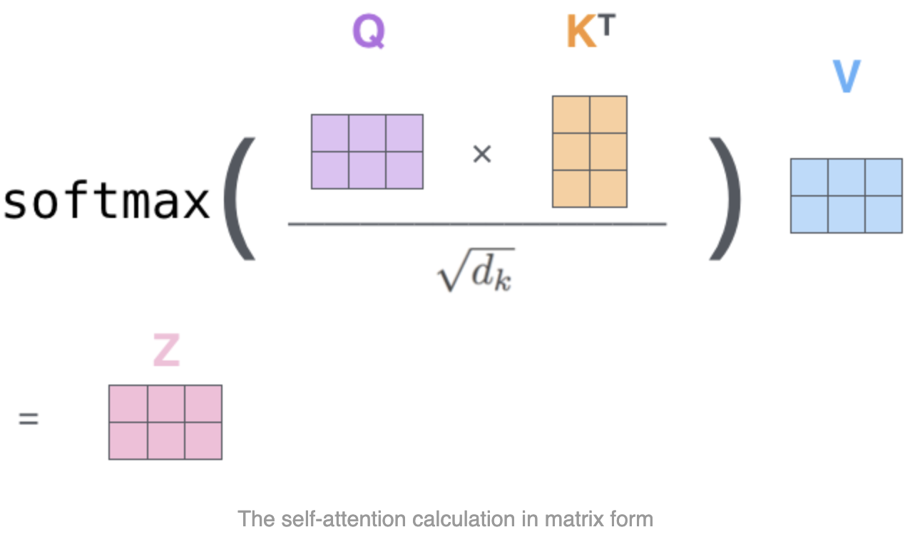
multi-head 拆分是在
dim维度,每个head的head_dim加总等于dim。拆分之后,att 的计算仅限于head_dim内部进行,也即上述公式中的 ${d_k}=head\_dim$,head 之间互不干涉。